Visualization
After processing your InSAR data, you have two powerful visualization options: an interactive GIS map viewer and detailed time-series plots. This guide covers both tools and their capabilities.
Interactive GIS Map Viewer
The gis_map_viewer.py script provides a web-based interface for exploring your change detection results.
Prerequisites
Ensure these files are present in your project directory:
change_detection_results.csv(required)binary_detection.tif(optional - GeoTIFF overlay)Basisdata_..._FGDB/folders (optional - historical data)
Launching the Viewer
| Bash | |
|---|---|
This starts a local web server and opens the map in your default browser.
Map Features
Interactive Elements
- Click Points: Click any detected change point for detailed information
- Layer Toggle: Show/hide different data layers
- Zoom Controls: Navigate to areas of interest
- Legend: Understand color coding and symbols
Information Panels
Each point displays: - Change magnitude and direction - Detection confidence - Temporal information - Coherence statistics - Original data source
Layer Options
- Change Points: Primary detection results
- GeoTIFF Overlay: Binary detection visualization
- Historical Data: Background reference layers
- Base Maps: Satellite imagery and street maps
Navigation Tips
Finding Significant Changes: - Use layer filters to show only high-confidence detections - Look for clustering patterns in urban areas - Check coastal and industrial regions
Exploring Details: - Click points for popup information - Use zoom to examine spatial patterns - Compare different time periods if available
Example Visualization
Here's an example of the detailed time-series analysis you can generate:
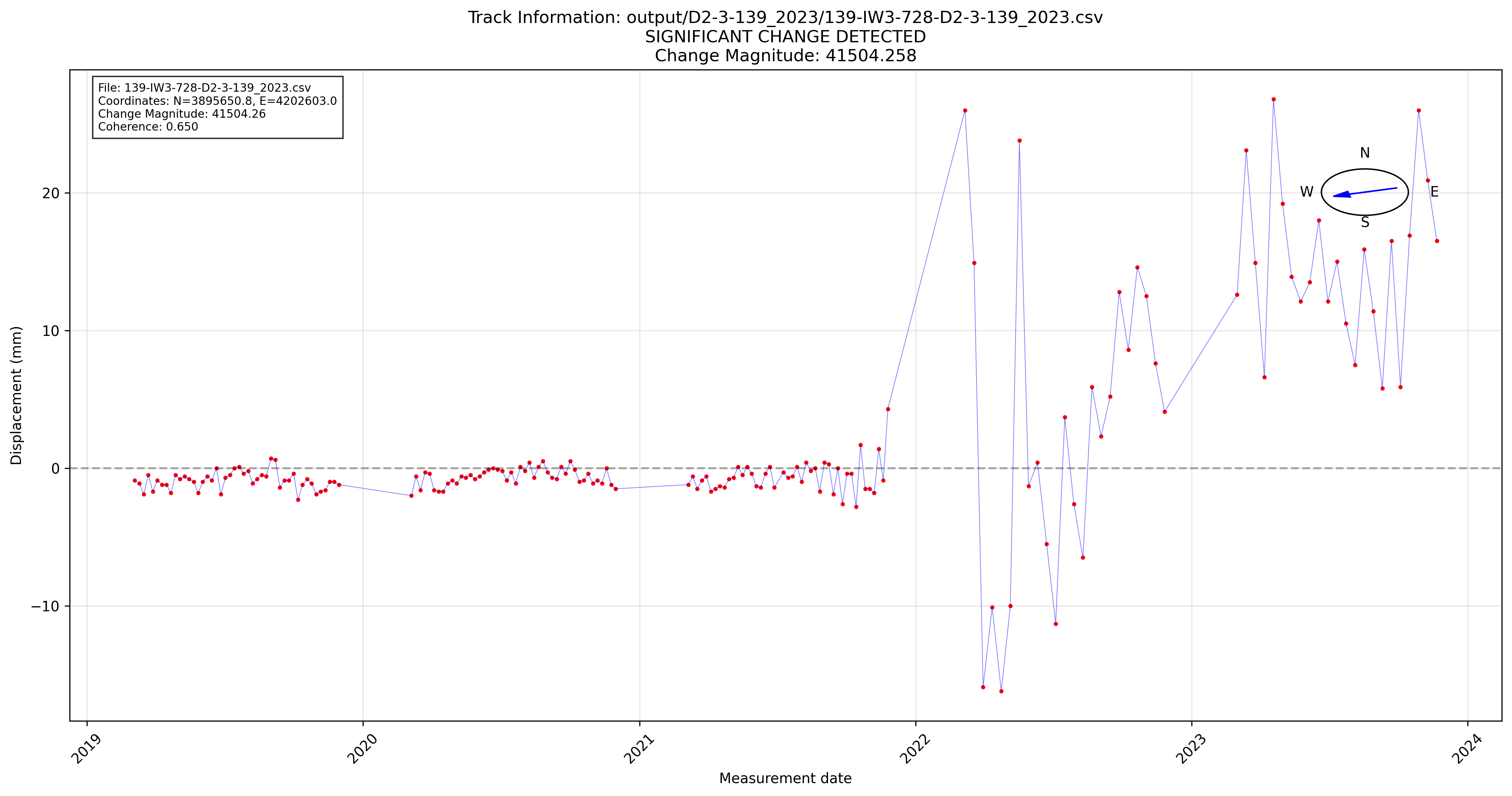
Figure: Time-series analysis showing significant ground motion change detected at point 20201 on Track 139. The plot displays displacement over time with clear indication of the change point detection.
This visualization demonstrates:
- Temporal progression of ground displacement measurements
- Change point detection algorithm results
- Statistical confidence intervals and thresholds
- Before/after analysis of the detected change
Time-Series Plots
The insar-visualizer.py script generates detailed static plots for specific points.
Basic Usage
| Bash | |
|---|---|
Parameters
--results
Path to the change detection results file.
| Bash | |
|---|---|
--num-points
Number of points to visualize for each category.
| Bash | |
|---|---|
--selection
Which points to visualize based on change magnitude:
highest: Largest change magnitudelowest: Smallest change magnitudemiddle: Medium change magnitudemixed: Combination of all categoriesall: All significant points
| Bash | |
|---|---|
--output-dir
Directory for saved plots (default: visualizations/).
| Bash | |
|---|---|
Plot Types Generated
Individual Point Plots
Each plot shows: - Time series: InSAR measurements over time - Change point: Detected change moment - Trend lines: Before and after velocities - Confidence intervals: Data uncertainty - Coherence overlay: Data quality indicators
Summary Statistics
- Change distribution: Histogram of detected changes
- Spatial patterns: Geographic distribution
- Temporal patterns: When changes occurred
- Quality metrics: Coherence and confidence statistics
Examples
High-Impact Changes
| Bash | |
|---|---|
Comprehensive Overview
| Bash | |
|---|---|
Quality Assessment
| Bash | |
|---|---|
Interpreting Visualizations
Map Viewer Insights
Spatial Patterns: - Clustered points may indicate localized processes - Linear patterns might suggest infrastructure effects - Isolated points could be individual events
Magnitude Distribution: - Large changes (red points) need immediate attention - Medium changes (yellow) require investigation - Small changes (green) may be monitoring priorities
Time-Series Analysis
Change Detection Quality: - Sharp transitions: Clear change events - Gradual transitions: Slow-onset processes - Noisy data: Lower confidence detections - Multiple changes: Complex temporal behavior
Velocity Analysis: - Acceleration: Increasing subsidence/uplift rates - Deceleration: Slowing ground motion - Reversal: Change from subsidence to uplift (or vice versa)
Advanced Visualization
Custom Analysis
For specialized analysis, you can:
- Filter Results: Select specific confidence or magnitude ranges
- Temporal Subsets: Focus on particular time periods
- Spatial Regions: Analyze specific geographic areas
- Quality Thresholds: Use only high-coherence data
Integration with GIS
Export results for use in professional GIS software:
Troubleshooting
Map Viewer Issues
Browser won't open:
- Manually navigate to http://localhost:5000
- Check firewall settings
- Try a different browser
Missing data layers: - Verify required files are in the correct directory - Check file permissions - Confirm file formats are correct
Slow performance: - Use fewer data points with filtering - Close other browser tabs - Restart the viewer
Plot Generation Issues
No plots generated: - Verify results file exists and has data - Check output directory permissions - Ensure sufficient disk space
Poor plot quality: - Increase figure resolution in code - Use different output formats (PNG, PDF) - Adjust plot styling parameters
Memory errors:
- Process fewer points at once
- Use --selection to limit data
- Close other applications
Best Practices
Workflow Integration
- Start with Map Viewer: Get overview of spatial patterns
- Identify Key Points: Focus on high-magnitude changes
- Generate Time Series: Analyze temporal behavior
- Document findings: Save plots and screenshots
- Validate Results: Cross-check with known events
Quality Control
- Always examine high-confidence detections first
- Compare multiple visualization methods
- Look for consistency in spatial and temporal patterns
- Validate against external information when available
Next Steps
- Explore Advanced Features for large-scale analysis
- Review the API Reference for detailed command options
- Check out Contributing to help improve the toolkit